Why Use R for Institutional Research? Part 1, Many Models

Introduction

I first heard about R when I was in graduate school in 2008 and fellow students used it to analyze their data. I didn’t bother to learn it at the time because, one, I didn’t see the benefit of it, and two, I assumed that without any programming experience, it was too difficult. So I continued with my same workflow: Clean data and make charts in Excel, import data into SPSS to analyze it, and then paste my output into a Word document and write up the results.

I started working in institutional research in 2013 and I still hadn’t made the switch to R, but was beginning to see the drawbacks of my workflow and the upside of coding. I often had to generate the same reports on a regular basis where the only thing that would change was the data. Or I’d have to generate the same charts or tables for each of the 15 colleges at the university, and on bad days, each of the 150-something majors. This quickly became unsustainable when I would, for example, get one of these requests late on a Friday afternoon and had to have it ready for a Board meeting on Monday. R increasingly seemed like a preferable alternative.

Fast-forward 7 years and my SPSS license has long since expired, I don’t recall the last time I made a chart in Excel, and the only thing I use Word for is making grocery lists. Today, my entire workflow exists inside of R.

In the intervening years, I have frequently met other institutional researchers who are stuck in the same mindset I was in 2008: For people who have never coded, R seems too overwhelming to learn, and even if they were to learn it, they do not see the benefits of doing so. In future posts I plan to address the former, but in this series of posts I want to address the latter: What’s the point of learning R for institutional research? Rather than list all of the reasons why R is an excellent choice for doing institutional research, I want to show examples of how I use it. In this post, I’ll demonstrate the scenario of using R to run many models.

If you are not an R user, do not worry about the details of the code below, but instead, pay attention to what the code is capable of producing.

Running One Model

Whether you want to predict future enrollment or explain why some students do not graduate, modeling is an important skill in institutional research. To show how to run a linear model in R, for all colleges and universities in the IPEDS Data Center, I downloaded their state, one year retention rates (i.e., the percent of first-time in college students who re-enroll their second fall term), student-faculty ratios, and the number of undergraduate applications they received for a given year. Here is the code for reading in the data and what the first five rows of data look like:

library(tidyverse)
library(broom)
library(drlib)

ipeds <- read_rds("processed-data/ipeds-sfr.rds")

head(ipeds, 5)

## # A tibble: 5 x 5
##   name                state   undergrad_applic… retention_rate student_faculty_…
##   <chr>               <chr>               <dbl>          <dbl>             <dbl>
## 1 Educational Techni… Puerto…                NA             11                21
## 2 A T Still Universi… Missou…                NA             NA                NA
## 3 Aaniiih Nakoda Col… Montana                NA             34                10
## 4 ABC Adult School    Califo…                NA             NA                 4
## 5 ABC Beauty Academy  Texas                  NA             25                10

In this contrived example, to build a linear model with retention rate as the outcome and student-faculty ratio and number of undergraduate applications as the predictors, I took the ipeds data frame, piped it (%>%) to the lm function, and then cleaned up the results with the tidy() function from the broom package. This gives us the model results:

ipeds %>% 
  lm(retention_rate ~ student_faculty_ratio + undergrad_applicants, data = .) %>% 
  tidy()

## # A tibble: 3 x 5
##   term                   estimate std.error statistic  p.value
##   <chr>                     <dbl>     <dbl>     <dbl>    <dbl>
## 1 (Intercept)           76.2      0.868         87.8  0.      
## 2 student_faculty_ratio -0.326    0.0589        -5.54 3.45e- 8
## 3 undergrad_applicants   0.000504 0.0000315     16.0  3.03e-54

At this point you may be thinking, “So what? I can just easily do the same thing in SPSS, or even Excel”. That is true, but what if instead of running one model, you had to run 150?

Running Many Models

As part of our university’s strategic business plan, I recently had to create separate models for each of the 150-something majors at the school. If I were still using SPSS, this would mean:

1. days of pointing and clicking and copying and pasting.
2. doing the same thing over and over again each time the project requirements changed, which is an inevitability.
3. having no documentation about the decisions I made because everything was done by pointing and clicking.

Returning to the original data set, let’s say I wanted repeat the same model above, but separately for each state. Using R, I first filter the data to only include states with at least 50 schools (an arbitrarily chosen cutoff point):

ipeds <- ipeds %>% 
  add_count(state) %>% 
  filter(n >= 50)

Next, I turn the model into a function:

state_regression <- function(df) {
 df %>% 
  lm(retention_rate ~ student_faculty_ratio + undergrad_applicants, data = .) 
}

From there, I can apply the function to each state in the data set, which returns a data frame with the model results for each state:

ipeds_model <- ipeds %>% 
  group_by(state) %>% 
  nest() %>% 
  mutate(model = map(data, state_regression),
         tidy_model = map(model, tidy)) %>% 
  unnest(tidy_model) 

head(ipeds_model, 5)

## # A tibble: 5 x 8
## # Groups:   state [2]
##   state            data model term         estimate std.error statistic  p.value
##   <chr>    <list<df[,5> <lis> <chr>           <dbl>     <dbl>     <dbl>    <dbl>
## 1 Puerto …    [146 × 5] <lm>  (Intercept)  87.5       5.80        15.1  2.48e-18
## 2 Puerto …    [146 × 5] <lm>  student_fac… -0.869     0.315       -2.76 8.68e- 3
## 3 Puerto …    [146 × 5] <lm>  undergrad_a…  0.00208   0.00140      1.49 1.45e- 1
## 4 Missouri    [171 × 5] <lm>  (Intercept)  84.5       5.46        15.5  1.91e-22
## 5 Missouri    [171 × 5] <lm>  student_fac… -1.07      0.458       -2.33 2.30e- 2

Now, with a separate model for each state all in a data frame, I can treat the model output like I would any other data. For example, here, I visualize the model results for each state:

ipeds_model %>% 
  filter(term != "(Intercept)") %>% 
  mutate(term = if_else(term == "student_faculty_ratio",
                        "Student/Faculty Ratio", "# of Undergraduate Applications")) %>% 
  ggplot(aes(x = reorder_within(state, -estimate, term),
             y = estimate,
             ymin = estimate - (2 * std.error),
             ymax = estimate + (2 * std.error))) +
  geom_pointrange(color = "grey60") +
  coord_flip() +
  guides(color = FALSE) +
  facet_wrap(~term, scales = "free", ncol = 2) +
  theme_classic() +
  scale_x_reordered() +
  geom_hline(yintercept = 0, linetype = 2) +
  labs(
    title = str_wrap("Is First-Year Retention Associated with Student-Faulty Ratio and/or Undergraduate Applications?", 75),
       subtitle = "Limited to states with at least 50 schools",
       caption = "Source: IPEDS Data Center",
       x = NULL, y = "Estimate")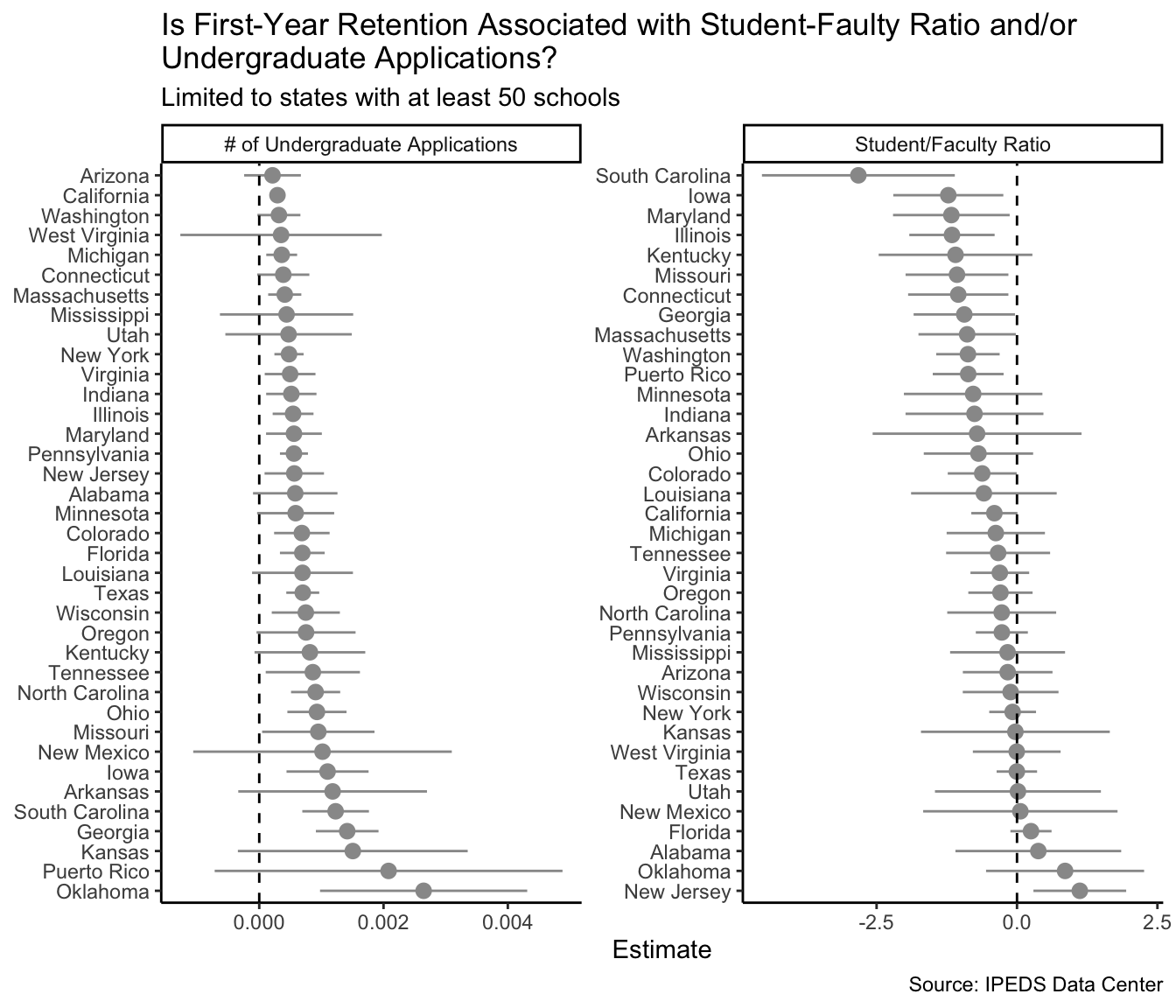

Conclusion

Claiming that there is more friction to learning R than there is to learning menu-driven tools is like saying learning to microwave TV dinners is easier than learning to cook the same meal from scratch. Both points might be true, but they obscure the ultimate goals of each: R, like cooking, unconstrains you, giving you the freedom to create whatever fills your imagination. And whether it’s running models for 150 majors or making soup for a large dinner party, learning to code and learning to cook can make your work not only more tenable, but more enjoyable, and in the long-run, simpler.