Tidying IPEDS Data in R

Reading in the Data

I first downloaded Fall 2012 to Fall 2018 distance education headcounts for every college and university in the IPEDS Data Center. In this first section, I read in the data, and display a subset of what the full data set looks like.

library(tidyverse)
library(scales)

theme_set(theme_light())

distance <- read_csv("raw-data/distance-fall-12-18.csv")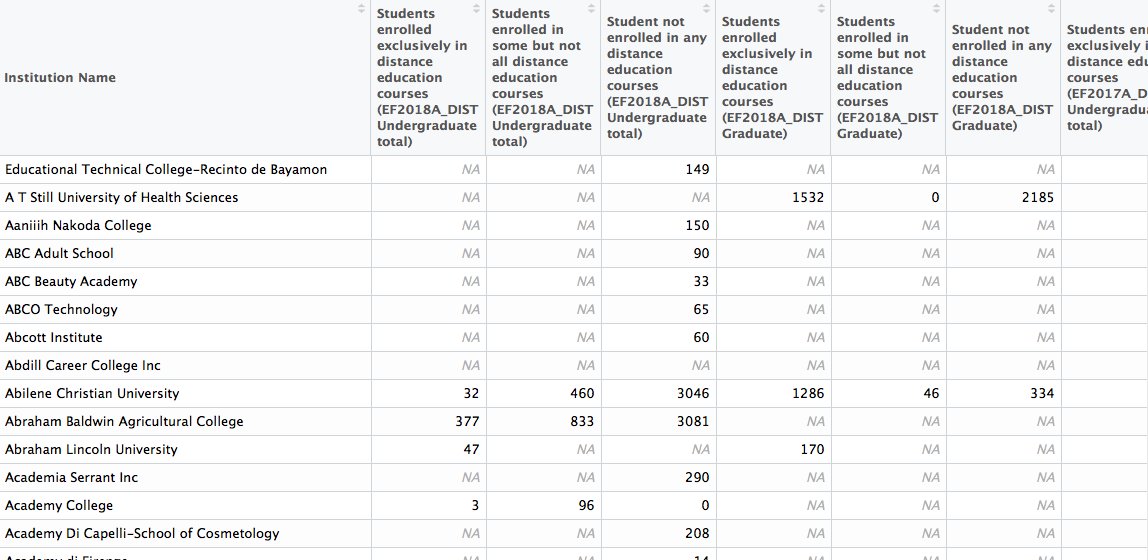

The data set contains 6,800 rows and 43 columns, and ignoring the Institution Name column, each of the remaining columns is some version of the following: Students enrolled exclusively in distance education courses (EF2018A_DIST Undergraduate total). Under that specific column, for each of the 6,800 institutions that reported data, are headcounts for exclusively distance undergraduate students in the fall term of 2018. The problem, thus, is that this column (and all the other ones like it) actually contains three pieces of information:

1. Level, which can take on the values undergraduate or graduate.
2. Modality, which can take on the values exlusively distance, some distance, or no distance.
3. Year, which can take on any integer value from 2012 to 2018.

This untidy format is exactly what makes IPEDS data tricky to work with. In contrast, tidy data - which means each variable is in its own column, each observation is in its own row, and each value is in its own cell¹ - is advantageous not just for working with data in R, but other software as well (e.g., pivot tables in Excel).

Tidying the Data

The first step to tidying this data is to pivot it so that all of the column names that contain the type of headcount are in one column, and the actual headcounts are in a different column. To do that, I use the gather()² function. I first provide gather() with the names of the two new variables that are being created - I call them variable and headcount, but they can be called anything you want - and then which columns I want pivoted from wide to long; here, I pivot everything from the 2nd column to the last column of the data set.

distance <- distance %>% 
  gather(variable, headcount, 2:ncol(.))

distance

## # A tibble: 285,600 x 3
##    `Institution Name`             variable                             headcount
##    <chr>                          <chr>                                    <dbl>
##  1 Educational Technical College… Students enrolled exclusively in di…        NA
##  2 A T Still University of Healt… Students enrolled exclusively in di…        NA
##  3 Aaniiih Nakoda College         Students enrolled exclusively in di…        NA
##  4 ABC Adult School               Students enrolled exclusively in di…        NA
##  5 ABC Beauty Academy             Students enrolled exclusively in di…        NA
##  6 ABCO Technology                Students enrolled exclusively in di…        NA
##  7 Abcott Institute               Students enrolled exclusively in di…        NA
##  8 Abdill Career College Inc      Students enrolled exclusively in di…        NA
##  9 Abilene Christian University   Students enrolled exclusively in di…        32
## 10 Abraham Baldwin Agricultural … Students enrolled exclusively in di…       377
## # … with 285,590 more rows

As you can see above, the data set now only has three columns, not 43. Same data, different layout. Looks better already, right?!?

We’re not done though. Remember, each row of the variable column contains three pieces of information: level, modality, and year. So for the next three steps I split that column apart so each of these variables are in their own column. First, I’ll make a new column for level.

There are countless ways of reaching the same endpoint in R, and in this instance, I use str_detect() to tell R to put “Undergraduate” in the level column if it detects the string “Undergraduate” in the variable column, and then perform the analogous task for “Graduate”.

distance <- distance %>% 
  mutate(level = case_when(
           str_detect(variable, "Undergraduate") ~ "Undergraduate",
           str_detect(variable, "Graduate") ~ "Graduate"))

distance

## # A tibble: 285,600 x 4
##    `Institution Name`          variable                        headcount level  
##    <chr>                       <chr>                               <dbl> <chr>  
##  1 Educational Technical Coll… Students enrolled exclusively …        NA Underg…
##  2 A T Still University of He… Students enrolled exclusively …        NA Underg…
##  3 Aaniiih Nakoda College      Students enrolled exclusively …        NA Underg…
##  4 ABC Adult School            Students enrolled exclusively …        NA Underg…
##  5 ABC Beauty Academy          Students enrolled exclusively …        NA Underg…
##  6 ABCO Technology             Students enrolled exclusively …        NA Underg…
##  7 Abcott Institute            Students enrolled exclusively …        NA Underg…
##  8 Abdill Career College Inc   Students enrolled exclusively …        NA Underg…
##  9 Abilene Christian Universi… Students enrolled exclusively …        32 Underg…
## 10 Abraham Baldwin Agricultur… Students enrolled exclusively …       377 Underg…
## # … with 285,590 more rows

See the new column on the end with level?

Next I do the same thing for modality: I tell R to look for specific strings, and make a new column based on those strings.

distance <- distance %>% 
         mutate(modality = case_when(
           str_detect(variable, "not enrolled in any") ~ "No Distance",
           str_detect(variable, "in some") ~ "Some Distance",
           str_detect(variable, "exclusively") ~ "Exclusively Distance"))

distance

## # A tibble: 285,600 x 5
##    `Institution Name`       variable                 headcount level  modality  
##    <chr>                    <chr>                        <dbl> <chr>  <chr>     
##  1 Educational Technical C… Students enrolled exclu…        NA Under… Exclusive…
##  2 A T Still University of… Students enrolled exclu…        NA Under… Exclusive…
##  3 Aaniiih Nakoda College   Students enrolled exclu…        NA Under… Exclusive…
##  4 ABC Adult School         Students enrolled exclu…        NA Under… Exclusive…
##  5 ABC Beauty Academy       Students enrolled exclu…        NA Under… Exclusive…
##  6 ABCO Technology          Students enrolled exclu…        NA Under… Exclusive…
##  7 Abcott Institute         Students enrolled exclu…        NA Under… Exclusive…
##  8 Abdill Career College I… Students enrolled exclu…        NA Under… Exclusive…
##  9 Abilene Christian Unive… Students enrolled exclu…        32 Under… Exclusive…
## 10 Abraham Baldwin Agricul… Students enrolled exclu…       377 Under… Exclusive…
## # … with 285,590 more rows

The last step of tidying is to get year in its own column. I could tell R to make a new variable and put “2012” if it detects “2012”, “2013” if it detects “2013”, and so-on, but there is a much simpler way: the parse_number() function, which drops any non-numeric characters from a string.

distance <- distance %>% 
  mutate(year = parse_number(variable))

The tidying is now done, and so although this next step isn’t necessary, renaming and reordering the variables and factor levels will make the data easier to work with.

# rename columns, reorder factor levels (e.g., Undergraduate before Graduate)
distance <- distance %>%
  select(institution_name = `Institution Name`, level,
         modality, year, headcount) %>% 
  mutate(level = fct_relevel(level, "Undergraduate"),
         modality = fct_relevel(modality, "Some Distance")) 

distance

## # A tibble: 285,600 x 5
##    institution_name                    level      modality        year headcount
##    <chr>                               <fct>      <fct>          <dbl>     <dbl>
##  1 Educational Technical College-Reci… Undergrad… Exclusively D…  2018        NA
##  2 A T Still University of Health Sci… Undergrad… Exclusively D…  2018        NA
##  3 Aaniiih Nakoda College              Undergrad… Exclusively D…  2018        NA
##  4 ABC Adult School                    Undergrad… Exclusively D…  2018        NA
##  5 ABC Beauty Academy                  Undergrad… Exclusively D…  2018        NA
##  6 ABCO Technology                     Undergrad… Exclusively D…  2018        NA
##  7 Abcott Institute                    Undergrad… Exclusively D…  2018        NA
##  8 Abdill Career College Inc           Undergrad… Exclusively D…  2018        NA
##  9 Abilene Christian University        Undergrad… Exclusively D…  2018        32
## 10 Abraham Baldwin Agricultural Colle… Undergrad… Exclusively D…  2018       377
## # … with 285,590 more rows

Behold, tidy data!

Visualizing the Data

With the data in a tidy format you can now do…pretty much whatever you want with it! In the examples below, I chose to visualize it, which demonstrates how - thanks to tidy data(!) - you can recycle the same code with slight alterations to make different plots. First, here are overall trends in distance education.

distance %>% 
  mutate(headcount = replace_na(headcount, 0)) %>% 
  group_by(year, modality) %>% 
  summarise(total = sum(headcount)) %>% 
  group_by(year) %>% 
  mutate(prop = total / sum(total)) %>% 
  ungroup() %>% 
  filter(modality != "No Distance") %>% 
  ggplot(aes(x = factor(year), y = prop, fill = modality)) +
  geom_col() +
  scale_y_continuous(label = percent_format()) +
  theme(legend.position = "top") +
  labs(x = "Fall Term", y = "% of Students",
       title = "Percentage of Students Enrolled in Distance Education",
       fill = NULL,
       subtitle = "Fall 2012 to Fall 2018",
       caption = "Source: IPEDS Data Center")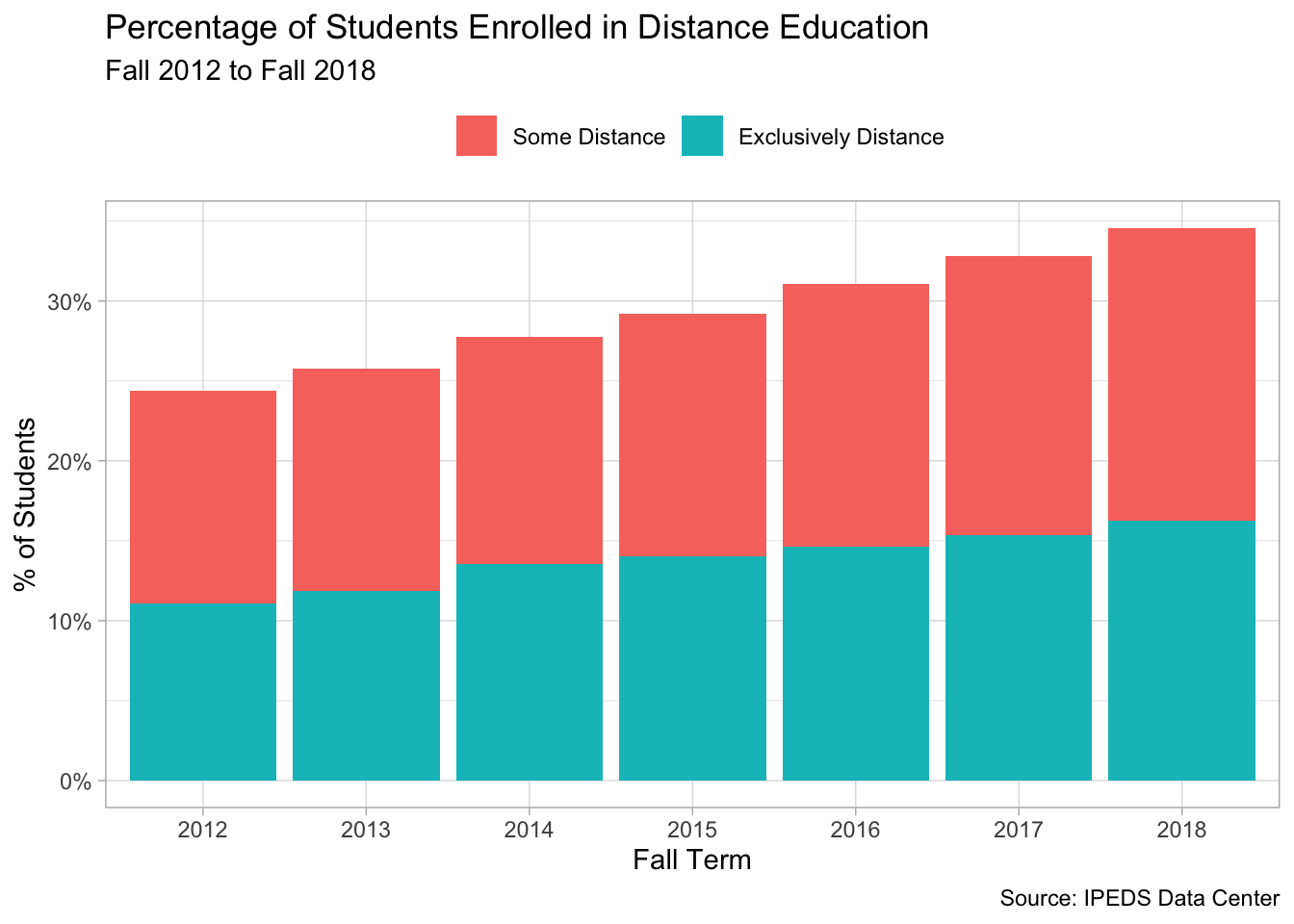

Next, I change the grouping variables to repeat the same chart except here I partition the data by level.

distance %>% 
  mutate(headcount = replace_na(headcount, 0)) %>% 
  group_by(year, modality, level) %>% 
  summarise(total = sum(headcount)) %>% 
  group_by(year, level) %>% 
  mutate(prop = total / sum(total)) %>% 
  ungroup() %>% 
  filter(modality != "No Distance") %>% 
  ggplot(aes(x = factor(year), y = prop, fill = modality)) +
  geom_col() +
  facet_wrap(~level) +
  scale_y_continuous(label = percent_format()) +
  theme(legend.position = "top") +
  labs(x = "Fall Term", y = "% of Students",
       title = "Percentage of Students Enrolled in Distance Education",
       fill = NULL,
       subtitle = "Fall 2012 to Fall 2018",
       caption = "Source: IPEDS Data Center")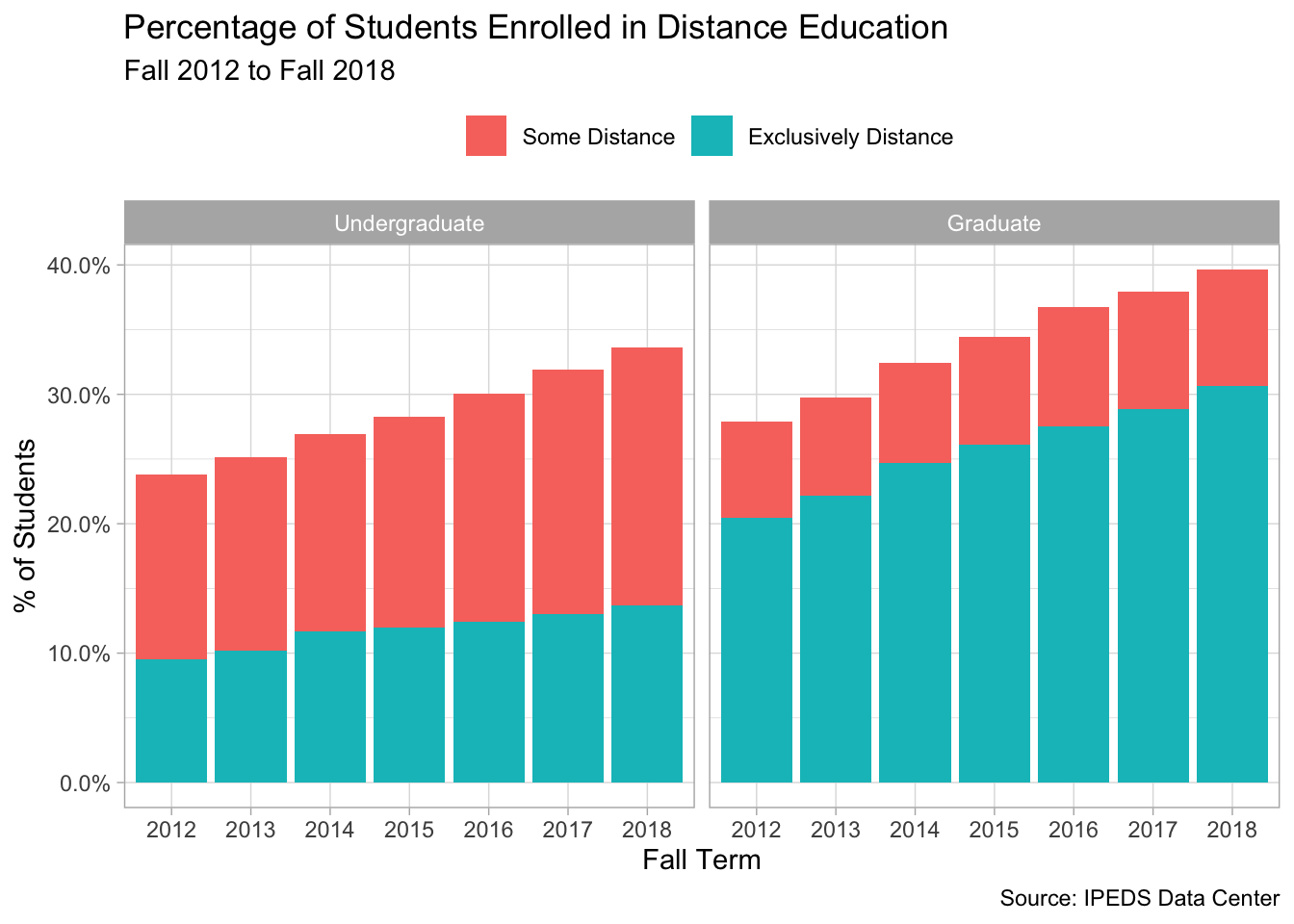

And once more, limiting the results to a single institution: Florida State University.

distance %>% 
  filter(institution_name == "Florida State University") %>% 
  mutate(headcount = replace_na(headcount, 0)) %>% 
  group_by(year, modality, level) %>% 
  summarise(total = sum(headcount)) %>% 
  group_by(year, level) %>% 
  mutate(prop = total / sum(total)) %>% 
  ungroup() %>% 
  filter(modality != "No Distance") %>% 
  ggplot(aes(x = factor(year), y = prop, fill = modality)) +
  geom_col() +
  facet_wrap(~level) +
  scale_y_continuous(label = percent_format()) +
  theme(legend.position = "top") +
  labs(x = "Fall Term", y = "% of Students",
       title = "Percentage of Florida State U. Students Enrolled in Distance Education",
       fill = NULL,
       subtitle = "Fall 2012 to Fall 2018",
       caption = "Source: IPEDS Data Center")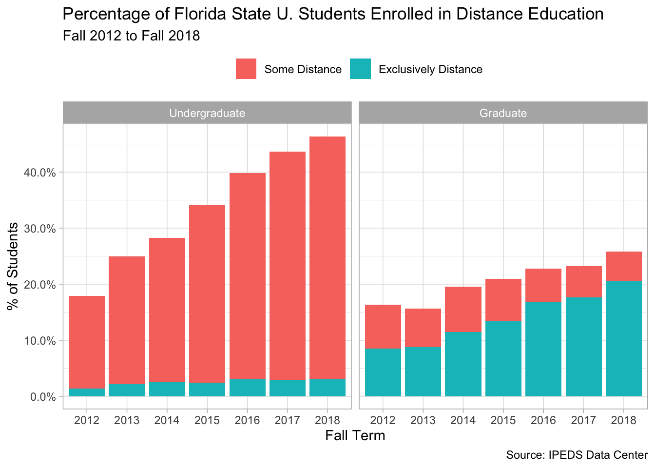

Conclusion

Among its many benefits, tidy data lets you devote more attention to what you want to do rather than how you want to do it. Yes, tidying data takes longer at the start, but in the long-run, it will save you time. In that way, it’s just like learning R!